Project TreeBeard
An Open Source Workflow to Identify and Quantify Forest Structural Diversity Patterns
Project Overview
The objective of Treebeard is to automate the classification and quantification of forest structural diversity from aerial imagery and LIDAR data in forested areas. The final product is intended to a be a free open-source QGIS plugin that runs on a python base as well as a series of Jupyter Notebooks that can be used for more customization. We are developing this workflow and tool in partnership with The Watershed Center. The Watershed Center conducts forest and watershed management activities throughout the St. Vrain Basin near Boulder, CO.
Identifying and quantifying forest structural diversity is an important part of their forestry practice planning and implementation. Forest structural diversity is a key component of forest ecosystem health, as forests that contain structural heterogeneity are critical for providing wildlife habitat and can be more resilient to natural disturbances. Being able to quantify forest structural heterogeneity is important to be able to assess the need for potential management actions, and it allows us to ensure that our forest management projects are creating structural heterogeneity rather than homogeneity. This tool will allow us to better determine the need for canopy gaps in project areas, and it will allow us to more accurately pinpoint beneficial locations for creating canopy gaps of various sizes when implementing projects.
For the purposes of this workflow and tool, we will be interested in using our current methods to evaluate the spatial heterogeneity in a several sites located within the Left Hand Creek watershed. We have developed workflows for two processes:
- Image classification/segmentation using the K-means algorithm and high resolution aerial imagery
- LIDAR data processing to generate a representation of forest canopy
The data generated by these processes will allow us to process and output spatial data representing the configuration of forest canopy and forest canopy gap polygons within a given study area. These polygons will be classified by acreage size categories.
This blog post will focus on the LIDAR workflow portion of the project.
The primary GitHub repostitory for the project is here.
LIDAR Overview
LIDAR, or Light Detection and Ranging, is a method of data collection that uses pulses of laser light to measure distances and identify the presence of solid objects. LIDAR sensors can be mounted on airborne platforms including aircraft and UAVs and can fly data collection missions over large areas. The output of LIDAR data collection can be used to create a three dimensional representation of physical objects, such as trees and vegetation, structures, bare ground, water surfaces, and other formations.
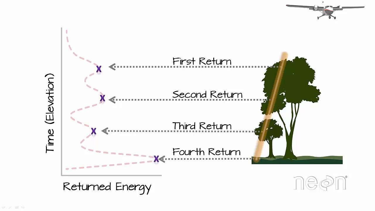
LIDAR provides a very valuable spatial data source, but the raw data can be quite cumbersome to process and work with. Each lidar pulse is classified as a specific "return" which corresponds to what type of structure the pulse is reflecting off of. These returns include "first returns" which represent the tallest structures the pulses reflect off of, such as tall tree canopy. "Intermediate returns" represented structures between the first returns and the ground. In the example of a forest, these returns represent leaves, branches, and smaller vegetation. "Last returns" or "ground returns" represent pulses reflecting off the bare ground. By processing these returns in different ways, we are able to generate digital elevation models that represent various structure configurations such as the bare ground elevation or the tree canopy elevation.
Study Site Overview
Left-hand Creek Watershed
Our primary study areas are located in the Left-hand Creek Watershed. The watershed serves as a significant ecological area that supports diverse plant and animal species and plays a crucial role in the local hydrological cycle.
The area is located within the Rocky Mountains to the north of Boulder, CO. It features mountainous terrain at a high elevation, with a continental climate that features large differences in day and night temperature due to high elevation. It is a highly wooded area, with some small rural developments found throughout. It is a home to a diverse set of plant and animal life. The area is currently undergoing restoration projects on some of its local streams.
import io
import os
import requests
import zipfile
import earthpy as et
import geopandas as gpd
import holoviews as hv
import hvplot as hv
import hvplot.pandas
import hvplot.xarray
import numpy as np
from pyproj import CRS
import rasterio
import rasterio.features
from rasterio.crs import CRS
import rioxarray as rxr
import rioxarray.merge as rxrm
from shapely.geometry import shape
from utils.process_lidar import process_canopy_areas
from utils.process_lidar import process_lidar_to_canopy
# Prepare project directories
# This project uses the EarthPy directory as the root path.
# You can specify your own root directory and paths below.
data_dir = os.path.join(et.io.HOME, et.io.DATA_NAME, 'treebeard')
lidar_dir = os.path.join(data_dir, 'lidar_tile_scheme_2020')
lidar_las_dir = os.path.join(data_dir, 'las_files')
os.makedirs(data_dir, exist_ok=True)
os.makedirs(lidar_dir, exist_ok=True)
os.makedirs(lidar_las_dir, exist_ok=True)
Functions
This workflow relies on two primary custom functions which are saved in the "utils" folder. They are included in the import statements above with the following lines of code:
from utils.process_lidar import process_canopy_areas
from utils.process_lidar import process_lidar_to_canopy
process_lidar_to_canopy
This function does the following:
- Lists all LAS files in the specified directory.
- Processes each LAS file to create DEMs from first and ground returns.
- Generates a canopy height DEM by subtracting the ground return DEM from the first return DEM.
- Classifies the canopy height into binary values (1 for canopy, 0 for no canopy).
- Merges and clips the processed DEMs to the specified project area.
- Converts the binary canopy mask into polygons and returns a GeoDataFrame of canopy areas.
process_canopy_area
This function performs the following steps:
- Validates and ensures that both the
canopy_gdfandstudy_areaGeoDataFrames have the same Coordinate Reference System (CRS). - Buffers the canopy geometries by the specified distance to account for spatial inaccuracies or to extend the canopy boundaries.
- Creates a new GeoDataFrame with the buffered geometries.
- Dissolves the buffered geometries into a single MultiPolygon to consolidate overlapping areas.
- Clips the dissolved canopy geometry to the study area boundary to restrict the data to the area of interest.
- Computes the difference between the study area and the clipped buffer to identify non-tree canopy areas.
- Explodes multipart polygons into individual geometries for detailed analysis of each gap.
- Calculates the area of each gap in acres and assigns size categories based on the gap size.
- Saves the processed GeoDataFrames as shapefiles to the specified output path, including:
- Buffered and clipped canopy areas
- Dissolved canopy
- Exploded canopy gaps with acreage and size categories
LIDAR Index Grid
Most LIDAR projects cover large geographic areas. In order to facilitate the organization and storage of the raw output of these data acquisition efforts, this data is often prepared in a grid of tiles. Each tile is smaller in size and easier to manage for smaller area of interest.
The following code downloads the LIDAR index grid for later use.
las_index_path = os.path.join(
data_dir,
lidar_dir,
'lidar_index_cspn_q2.shp'
)
# Download LIDAR index tiles
# Specify the download URL for the LAS tile index if it exists
# This example is downloading LIDAR from DRCOG 2020 LIDAR located at this path:
# 'https://lidararchive.s3.amazonaws.com/2020_CSPN_Q2/'
# Modify this the URL below with a LIDAR tile index for a particular LIDAR project
if not os.path.exists(las_index_path):
las_index_url = ('https://gisdata.drcog.org:8443/geoserver/DRCOGPUB/'
'ows?service=WFS&version=1.0.0&request=GetFeature&'
'typeName=DRCOGPUB:lidar_index_cspn_q2&outputFormat=SHAPE-ZIP')
# Download the ZIP file
response = requests.get(las_index_url)
response.raise_for_status() # Check that the request was successful
# Extract the ZIP file
with zipfile.ZipFile(io.BytesIO(response.content)) as zip_ref:
zip_ref.extractall(lidar_dir)
las_index_gdf = (
gpd.read_file(las_index_path).set_index('tile')
# .loc[['N3W345']]
)
# Project to EPSG 4269 for plotting
las_index_gdf = las_index_gdf.to_crs('EPSG:4326')
crs = las_index_gdf.crs
las_index_plot = las_index_gdf.hvplot(
tiles = 'OSM',
crs=las_index_gdf.crs,
geo = True,
line_color='black',
line_width=2,
fill_alpha=0
)
las_index_plot
Study Areas
The following code processes the study area shapefile. This shapefile should contain a column called "Proj_ID" which includes values representing names of the study areas.
# Open project areas shapefile and plot
# Save your study area shapefile as zipfile at the path in proj_zip_path
proj_zip_path = 'assets/project_areas_merged.zip'
with zipfile.ZipFile(proj_zip_path, 'r') as zip_ref:
temp_dir = '/tmp/extracted_shapefile' # You can specify any temporary directory
zip_ref.extractall(temp_dir)
extracted_shapefile_path = temp_dir + '/'
proj_area_gdf = gpd.read_file(extracted_shapefile_path)
proj_area_gdf = proj_area_gdf.to_crs("EPSG:4326")
proj_area_plot = proj_area_gdf.hvplot(
x='x',
y='y',
aspect='equal',
tiles='OSM',
geo=True,
line_color='red',
line_width=2,
fill_alpha=0
)
proj_area_plot
Identify Relevant LIDAR Tiles
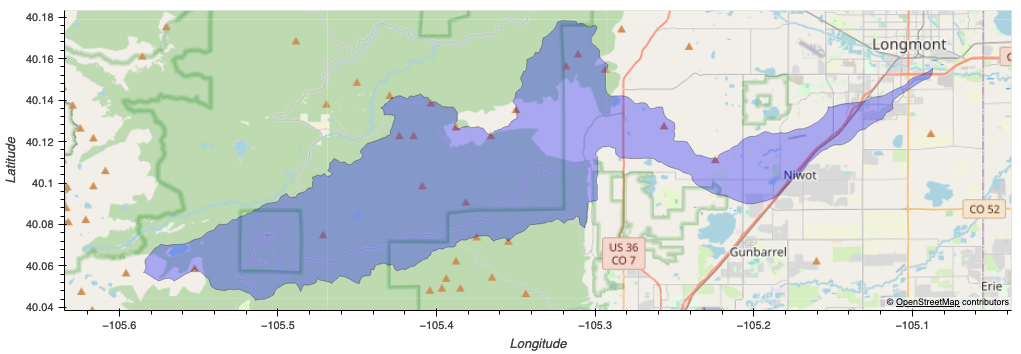
The following code overlays the LIDAR index grid with the study areas in order to identify the tiles which need to be downloaded and processed.
# Identify the tiles that intersect each project area
select_tiles_gdf = gpd.sjoin(las_index_gdf, proj_area_gdf, how='inner', predicate='intersects')
select_tiles_gdf.reset_index(drop=False)
select_tile_plot = select_tiles_gdf.hvplot(
x='x',
y='y',
aspect='equal',
geo=True,
line_color='blue',
line_width=2,
fill_alpha=0,
xaxis=None,
yaxis=None
)
tile_proj_plot = select_tile_plot * proj_area_plot
#hv.save(tile_proj_plot, 'lidar_tile_plot.png')
tile_proj_plot
select_tiles_gdf = select_tiles_gdf.reset_index(drop=False)
# Generate list of all tiles per project area
tiles_by_area = select_tiles_gdf.groupby('Proj_ID')['tile'].apply(list).reset_index()
tiles_by_area
| Proj_ID | tile | |
|---|---|---|
| 0 | Conifer Hill | [N4W399, N4W397, N4W389, N4W396, N4W388, N4W29... |
| 1 | Unnamed 1 | [N4W264] |
| 2 | Unnamed 2 | [N4W381, N4W391] |
| 3 | Zumwinkel | [N4W351] |
Download and Process LIDAR Tiles
The following code downloads the .las files that overlap with a specified study area by name. These tiles are used by the process_lidar_to_canopy function to generate a geodataframe of canopy within the study area. By default, this identifies canopy taller than 5' above the ground but this parameter can be adjusted.
# Download and process .las tiles for the desired study area
# This code assumes you have prepared a study area shapefile
# with a column called 'Proj_ID' that specifies the name of the study area.
# This is downloading .las files from the URL below. Adjust for a different LIDAR project
las_root_url = 'https://lidararchive.s3.amazonaws.com/2020_CSPN_Q2/'
# Set the project name here
proj_area = proj_area_gdf[proj_area_gdf['Proj_ID'] == 'Zumwinkel']
# Create output folder for study area being used
proj_area_name = proj_area['Proj_ID'].iloc[0]
lidar_download_path = os.path.join(data_dir, proj_area_name, "las_files")
if not os.path.exists(lidar_download_path):
os.makedirs(lidar_download_path)
# Download .las tiles for study area
site_to_process = tiles_by_area[tiles_by_area['Proj_ID'] == proj_area_name].copy()
for index, row in site_to_process.iterrows():
tiles = row['tile']
sel_proj_area_gdf = proj_area_gdf[proj_area_gdf['Proj_ID'] == proj_area_name]
# Download all tiles for project area, process, and clip/merge
tile_agg = []
print("Processing LIDAR for " + proj_area_name)
for tile in tiles:
file_name = tile + ".las"
print("Processing LIDAR tile " + tile)
tile_path = os.path.join(
lidar_download_path,
file_name
)
download_url = las_root_url + tile + ".las"
if not os.path.exists(tile_path):
# Download the LAS file
response = requests.get(download_url)
# Check if the request was successful
if response.status_code == 200:
with open(tile_path, 'wb') as file:
file.write(response.content)
print(f"File downloaded successfully and saved to {tile_path}")
else:
print(f"Failed to download file. Status code: {response.status_code}")
canopy_gdf = process_lidar_to_canopy(proj_area, lidar_download_path, canopy_height=5)
Process Canopy into Output Shapefiles
This code uses the process_canopy_area function to convert the canopy geodataframe into processed output shapefiles representing canopy, buffered canopy, and canopy gaps. We apply a buffer to the canopy to clean up "noise" within the canopy areas that represent small gaps between branches and leaves. We also expand the area around the edge of canopy to account for variation in tree structure and dripline. This buffered canopy area is used to clip the study area - all remaining areas represent gaps.
# Process output shapefiles
output_path = os.path.join(data_dir, proj_area_name, "processed_output_files")
if not os.path.exists(output_path):
os.makedirs(output_path)
process_canopy_areas(canopy_gdf, proj_area, output_path, buffer_distance=5)
Plot of Processed Data
The plot below shows both process canopy areas and processed gap areas.
# Plot outputs of canopy and buffered gaps
gaps_filename = "lidar_" + proj_area_name + "_canopy_gaps_calced.shp"
gaps_shp_path = os.path.join(output_path, gaps_filename)
canopy_gaps_calced = gpd.read_file(gaps_shp_path)
canopy_gaps_calced_to_plot = canopy_gaps_calced.to_crs("EPSG:4326")
gaps_plot = canopy_gaps_calced_to_plot.hvplot(
x='x',
y='y',
aspect='equal',
geo=True,
line_color='blue',
line_width=2,
fill_alpha=.5,
width = 600,
height=600,
tiles = 'EsriImagery',
title = "Processed Canopy Gaps from LIDAR with 5' Buffer"
)
canopy_gdf_to_plot = canopy_gdf.to_crs("EPSG:4326")
canopy_plot = canopy_gdf_to_plot.hvplot(
x='x',
y='y',
aspect='equal',
geo=True,
line_color='blue',
line_width=2,
fill_alpha=.5,
width = 600,
height=600,
tiles = 'EsriImagery',
title = "Processed Canopy from LIDAR"
)
gaps_plot + canopy_plot